The article studies the advantage of Support Vector Regression (SVR) over Simple Linear Regression (SLR) models for predicting real values, using the same basic idea as Support Vector Machines (SVM) use for classification.
The article studies the advantage of Support Vector Regression (SVR) over Simple Linear Regression (SLR) models. SVR uses the same basic idea as Support Vector Machine (SVM), a classification algorithm, but applies it to predict real values rather than a class. SVR acknowledges the presence of non-linearity in the data and provides a proficient prediction model. Along with the thorough understanding of SVR, we also provide the reader with hands on experience of preparing the model on R. We perform SLR and SVR on the same dataset and make a comparison. The article is organized as follows; Section 1 provides a quick review of SLR and its implementation on R. Section 2 discusses the theoretical aspects of SVR and the steps to fit SVR on R. It also covers the basics of tuning SVR model. Section 3 is the conclusion.
Simple Linear Regression (SLR)
Simple Linear Regression (SLR) is a statistical method that examines the linear relationship between two continuous variables, X and Y. X is regarded as the independent variable while Y is regarded as the dependent variable. SLR discovers the best fitting line using Ordinary Least Squares (OLS) criterion. OLS criterion minimizes the sum of squared prediction error. Prediction error is defined as the difference between actual value (Y) and predicted value (Ŷ) of dependent variable. OLS minimizes the squared error function defined as follows:

SLR minimizes the Squared Errors (SE) to optimize the parameters of a linear model, αi and βi, thereby computing the best-fit line, which is represented as follows:

Let us perform SLR on a sample data, with a single independent variable. We treat X as the independent variable and Y as the dependent variable. The data is in .csv format and can be downloaded by clicking here.
Now we use R to perform the analysis. The R script is provided side by side and is commented for better understanding of the reader. We start with the scatter plot shown in Figure 1. Please set the working directory in R using setwd( ) function and keep sample data in the working directory.
## Prepare scatter plot

#Read data from .csv file
data=read.csv("SVM.csv", header=T)
head(data)

#Scatter Plot
plot(data, main ="Scatter Plot")
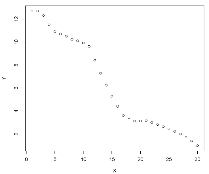
Figure 1: Scatter plot.
The first step is to visualize the data to obtain basic understanding. The scatter plot suggests negative relationship between X and Y. Let us try fitting line on the scatter plot using Ordinary Least Squares (OLS) method.
## Add best-fit line to the scatter plot

#Fit linear model using OLS
model=lm(Y~X,data)

#Overlay best-fit line on scatter plot
abline(model)
We expect a negative relationship between X and Y. Equation (3) represents the linear model fitting our sample data. The values of Y, dependent variable, are obtained by plugging in the given values of X, independent variable.

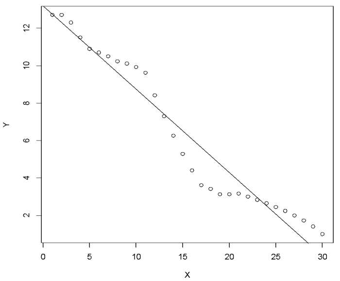
Figure 2: Overlay best-fit line on scatter plot.
Figure 2 shows the best-fit line of our data set. It can be observed that a linear fit is not able to capture the complete relationship between X and Y. In fact, no model can capture the complete relationship in a statistical relation. The idea is to strive for a reasonable prediction. The next step would be to evaluate the fitted model. One of the widely used methods for assessing statistical models is Root Mean Square Error (RMSE). It quantifies the performance of a regression model. It measures the root of mean of squared errors and is calculated as shown in equation (4). The lower value of RMSE implies that the prediction is close to actual value, indicating a better predictive accuracy.

Before calculating RMSE for our example, let us look at the predicted values as estimated by the linear model. The actual values are shown in black while the predicted values are show in blue in Figure 3. The R code is as follows:
## Scatter plot displaying actual values and predicted values

#Scatter Plot
plot (data, pch=16)

#Predict Y using Linear Model
predY <- predict (model, data)

#Overlay Predictions on Scatter Plot
points (data$X, predY, col = "blue", pch=16)
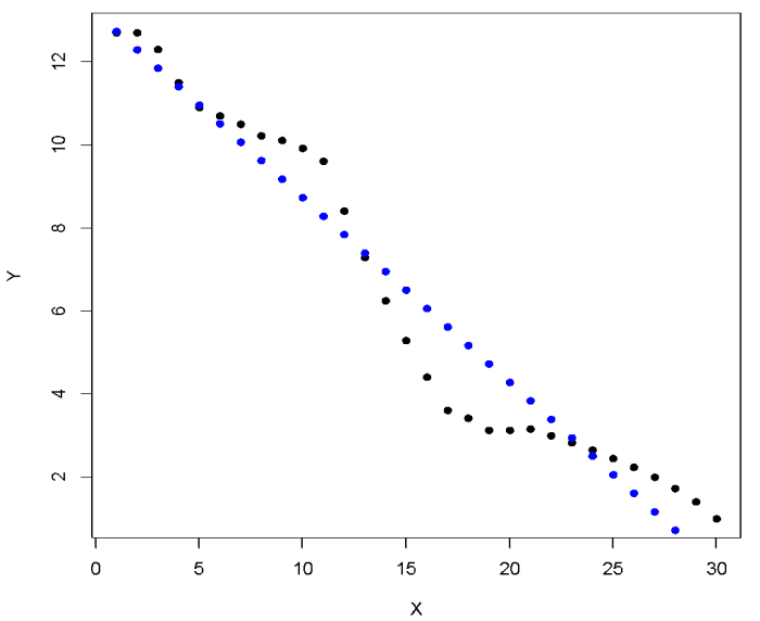
Figure 3: Actual values vs. predicted values (blue) using SLR.
Figure 3 provides a better understanding of RMSE. Ŷi and Yi in RMSE (equation 3) are blue and black dots respectively. The vertical distance between black and corresponding blue dot is the error term (ϵi). Let us now calculate RMSE for the linear model. In order to calculate RMSE in R, “hydroGOF” package is required. R code is as follows:
## RMSE Calculation for linear model

#Install Package
install.packages("hydroGOF")

#Load Library
library(hydroGOF)

#Calculate RMSE
RMSE=rmse(predY,data$Y)
The computation using above R code shows RMSE to be 0.94 for the linear model. The absolute value of RMSE does not reveal much, but a comparison with alternate models adds immense value. We will try to improve RMSE using Support Vector Regression (SVR) but before that let us understand the theoretical aspects of SVR.
Support Vector Regression (SVR)
Support Vector Regression (SVR) works on similar principles as Support Vector Machine (SVM) classification. One can say that SVR is the adapted form of SVM when the dependent variable is numerical rather than categorical. A major benefit of using SVR is that it is a non-parametric technique. Unlike SLR, whose results depend on Gauss-Markov assumptions, the output model from SVR does not depend on distributions of the underlying dependent and independent variables. Instead the SVR technique depends on kernel functions. Another advantage of SVR is that it permits for construction of a non-linear model without changing the explanatory variables, helping in better interpretation of the resultant model. The basic idea behind SVR is not to care about the prediction as long as the error (ϵi) is less than certain value. This is known as the principle of maximal margin. This idea of maximal margin allows viewing SVR as a convex optimization problem. The regression can also be penalized using a cost parameter, which becomes handy to avoid over-fit. SVR is a useful technique provides the user with high flexibility in terms of distribution of underlying variables, relationship between independent and dependent variables and the control on the penalty term. Now let us fit SVR model on our sample data. R package “e1071” is required to call svm function. R code is as follows:
## Fit SVR model and visualize using scatter plot

#Install Package
install.packages("e1071")

#Load Library
library(e1071)

#Scatter Plot
plot(data)

#Regression with SVM
modelsvm = svm(Y~X,data)

#Predict using SVM regression
predYsvm = predict(modelsvm, data)

#Overlay SVM Predictions on Scatter Plot
points(data$X, predYsvm, col = "red", pch=16)
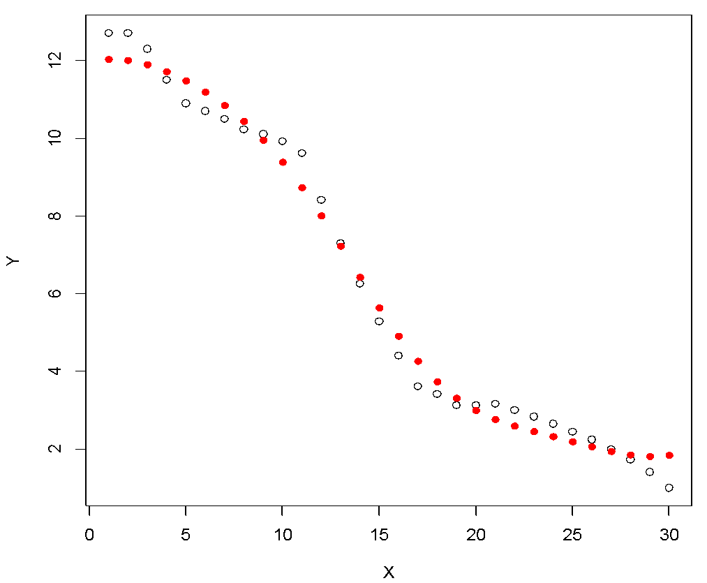
Figure 4: Actual values (white) vs. predicted values (red) using SVR.
The white dots ad the red dots represent actual values and predicted values respectively. At first glance, the SVR model looks much better compared to SLR model as the predicted values are closer to the actual values. To obtain to a better understanding, let us try to understand and represent the constructed model.
SVR technique relies on kernel functions to construct the model. The commonly used kernel functions are: a) Linear, b) Polynomial, c) Sigmoid and d) Radial Basis. While implementing SVR technique, the user needs to select the appropriate kernel function. The selection of kernel function is a tricky and requires optimization techniques for the best selection. A discussion on kernel selection is outside the scope of discussion for this article. In the constructed SVR model, we used the automated kernel selection provided by R. Radius Basis Function (RBF) kernel is used in the above model. Given a non-linear relation between the variables of interest and difficulty in kernel selection, we would suggest the beginners to use RBF as the default kernel. The kernel function transforms our data from non-linear space to linear space. The kernel trick allows the SVR to find a fit and then data is mapped to the original space. Now let us represent the constructed SVR model:

The value of parameters W and b for our data is -4.47 and -0.06 respectively. The R code to calculate parameters is as follows:
##Calculate parameters of the SVR model

#Find value of W
W = t(modelsvm$coefs) %*% modelsvm$SV

#Find value of b
b = modelsvm$rho
We have learnt that the real value of RMSE lies is comparison of alternative models. In the SVR model, the predicted values are closer to the actual values, suggesting a lower RMSE value. RMSE calculation would allow us to compare the SVR model with the earlier constructed linear model. A lower value of RMSE for SVR model would confirm that the performance of SVR model is better than that of SLR model. The R code for RMSE calculation is as follows:
## RMSE for SVR Model

#Calculate RMSE
RMSEsvm=rmse(predYsvm,data$Y)
RMSE for SVR model is 0.433, much lower than 0.94 computed earlier for the SLR model. By default svm function in R considers maximum allowed error (ϵi) to be 0.1. In order to avoid over-fitting, the svm SVR function allows us to penalize the regression through cost function. The SVR technique is flexible in terms of maximum allowed error and penalty cost. This flexibility allows us to vary both these parameters to perform a sensitivity analysis in attempt to come up with a better model. Now we will perform sensitivity analysis, by training a lot of models with different allowable error and cost parameter. This process of searching for the best model is called tuning of SVR model. The R code for tuning of SVR model is as follows:
## Tuning SVR model by varying values of maximum allowable error and cost parameter

#Tune the SVM model
OptModelsvm=tune(svm, Y~X, data=data,ranges=list(elsilon=seq(0,1,0.1), cost=1:100))

#Print optimum value of parameters
print(OptModelsvm)

#Plot the perfrormance of SVM Regression model
plot(OptModelsvm)
The above R code tunes the SVR model by varying maximum allowable error and cost parameter. The tune function evaluates performance of 1100 models (100*11) i.e. for every combination of maximum allowable error (0 , 0.1 , . . . . . 1) and cost parameter (1 , 2 , 3 , 4 , 5 , . . . . . 100). The OptModelsvm has value of epsilon and cost at 0 and 100 respectively. The plot below visualizes the performance of each of the model. The legend on the right displays the value of Mean Square Error (MSE). MSE is defined as (RMSE)2 and is also a performance indicator.
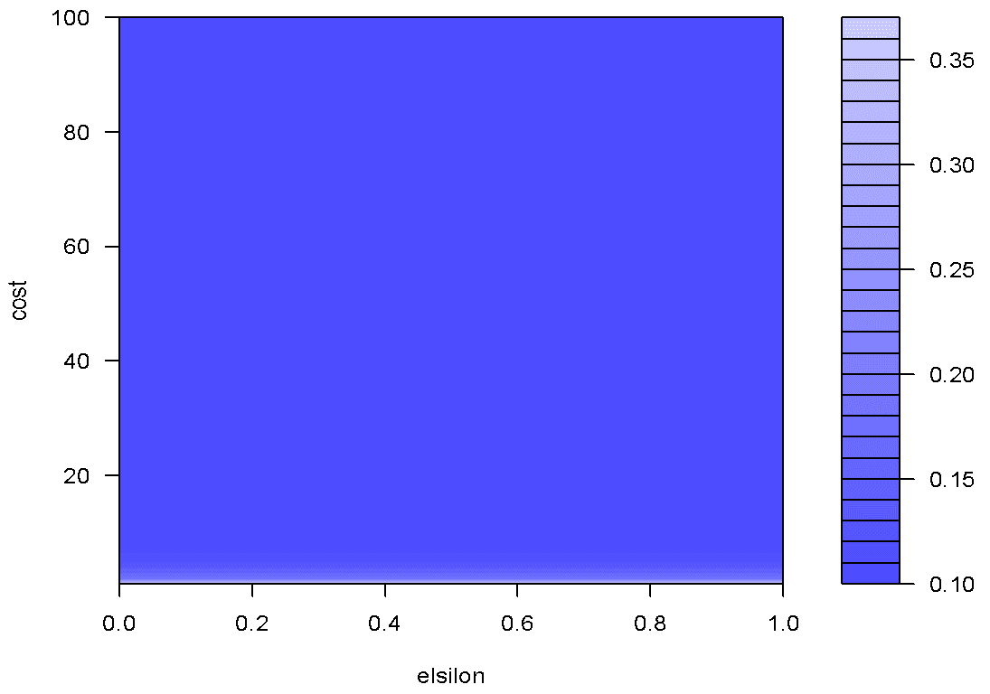
Figure 5: Performance of SVM.
The best model is the one with lowest MSE. The darker the region the lower the MSE, which means better the model. In our sample data MSE is lowest at epsilon – 0 and cost – 7. We do not have to do this step manually, R provides us with the best model from the set of trained models. The R code to select the best model and compute RMSE is as follows:
## Select the best model out of 1100 trained models and compute RMSE

#Find out the best model
BstModel=OptModelsvm$best.model

#Predict Y using best model
PredYBst=predict(BstModel,data)

#Calculate RMSE of the best model
RMSEBst=rmse(PredYBst,data$Y)
The RMSE for the best model is 0.27, which is much lower than 0.43, RMSE of earlier fitted SVR model. We have successfully tuned the SVR model.
The next step is to represent the tuned SVR model. The value of parameters W and b the tuned model is -5.3 and -0.11 respectively. The R code to calculate parameters is as follows:
##Calculate parameters of the Best SVR model

#Find value of W
W = t(BstModel$coefs) %*% BstModel$SV

#Find value of b
b = BstModel$rho
A comparison of RMSE for the constructed SVR models, SVR and tuned SVR helps us to select the best model. Let us now visualize both these models in a single plot to enhance our understanding. Figure 7 displays the combined plot. The R code is as follows:
## Plotting SVR Model and Tuned Model in same plot

plot(data, pch=16)
points(data$X, predYsvm, col = "blue", pch=3)
points(data$X, PredYBst, col = "red", pch=4)
points(data$X, predYsvm, col = "blue", pch=3, type="l")
points(data$X, PredYBst, col = "red", pch=4, type="l")
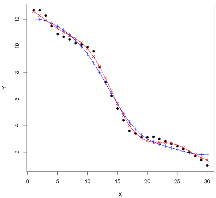
Figure 6: Actual data (black), SVR model (blue), tuned SVR model (red).
The tuned SVR model (red) fits the sample data much better than earlier developed SVR model. We hope that this tutorial on Support Vector Regression (SVR) was useful. Please download the complete code by clicking here. We have provided code for each of the steps.
Conclusion
The article discusses the basic concepts of Simple Linear Regression (SLR) and Support Vector Regression (SVR). SVR is a useful and flexible technique, helping the user to deal with the limitations pertaining to distributional properties of underlying variables, geometry of the data and the common problem of model overfitting. The choice of kernel function is critical for SVR modeling. We recommend beginners to use linear and RBF kernel for linear and non-linear relationship respectively.
We observe that SVR is superior to SLR as a prediction method. SLR cannot capture the nonlinearity in a dataset and SVR becomes handy in such situations. We find that SVR provides a good fit on nonlinear data. We also compute Root Mean Square Error (RMSE) for both SLR and SVR models to evaluate performance of the models.
Further, we explain the idea of tuning SVR model. Tuning of SVR model can be performed as the technique provides flexibility with respect to maximum error and penalty cost. Tuning the model is extremely important as it optimizes the parameters for best prediction. In the end we compare the performance of SLR, SVR and tuned SVR model. As expected, the tuned SVR model provides the best prediction.
